Checking fit results
The fastest way to check the results of your fit is to use the fit_scrutinizer program. This program has graphical user interface (GUI) that lets you select each parameter of each component, and see the image of that parameter at the same time showing the spectrum of a particular spaxel. After installation of IFSCube by the pip installer, fit_scrutinizer will be appended to your path, making it accessible from any directory directly from the command line.
For instance, let us take a look at that first attempt at a data cube fit, saved as myfit.fits. The data cube that originated it is the ngc3081_cube.fits, therefore the calling sequence to fit_scrutinizer should read
fit_scrutinizer ngc3081_cube_linefit.fits
This will start a GUI similar to the one in the figure below, but without any of the plots yet. To start plotting your results you have to select a parameter from the list at the lower left corner, and a component from the list right next to it. In this example we selected the velocity for the only component available, component “0”. Next we click “Image plot” to generate the image of the velocity for the first component in the upper left.
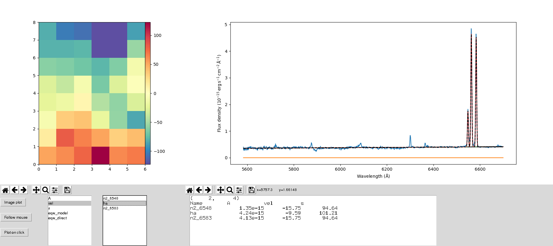
Example of the interface of the fit_scrutinizer program, showing the velocity image, and the spectrum in the spaxel (2, 4).
At this point only the image is visible, but no spectral plot will be produced until you click on either “Follow mouse” or “Plot on click”. The former will cause a new spectral plot to be generated every time the mouse enters a new spaxel on the image at the upper left, while the latter will only plot the spectrum when you click on a spaxel.
The output file
The output file generated by cubefit is a Multi-Extension FITS file (MEF), consisting of images and tables that store the results of the fitting process. This file can be accessed by any program capable of dealing with the FITS format.
Let us start by taking a look at the extensions that are present in the output file of the example fit for ’ngc3081_cube.fits’. If you have not changed the example configuration file, the output file should be named ’ngc3081_cube_linefit.fits’. I recommend opening a interactive python interpreter, such as ipython, and entering the following commands:
from astropy.io import fits

cube = fits.open('ngc3081_cube_linefit.fits')

cube.info()
The output should read:
Filename: ngc3081_cube_linefit.fits
No.    Name      Ver    Type      Cards   Dimensions   Format
  0  PRIMARY       1 PrimaryHDU      70   ()
  1  FITSPEC       1 ImageHDU        13   (6, 8, 1660)   float64
  2  FITCONT       1 ImageHDU        13   (6, 8, 1660)   float64
  3  STELLAR       1 ImageHDU        13   (6, 8, 1660)   float64
  4  MODEL         1 ImageHDU        13   (6, 8, 1660)   float64
  5  SOLUTION      1 ImageHDU        17   (6, 8, 10)   float64
  6  EQW_M         1 ImageHDU        17   (6, 8, 3)   float64
  7  EQW_D         1 ImageHDU        17   (6, 8, 3)   float64
  8  STATUS        1 ImageHDU        16   (6, 8)   int64
  9  MASK2D        1 ImageHDU        16   (6, 8)   int64
  10  SPECIDX       1 BinTableHDU     13   48R x 2C   ['K', 'K']
  11  PARNAMES      1 BinTableHDU     13   9R x 2C   [7A, 2A]
  12  FITCONFIG     1 BinTableHDU     13   39R x 2C [64A, 64A])
There are 13 extensions within the output file, and I will now explain briefly what each of them contains.
- PRIMARY: This is just a copy of the original header extension of the input file. Ideally this should have a good description of what the science data is.
- FITSPEC: A copy of the input science data, without any changes other than a trimming to the given fitting window. It has dimensions of (columns, rows, wavelength).
- FITCONT: If a continuum was fit to the data, this extension will contain the values of that pseudo-continuum at each wavelength coordinate.
- STELLAR: The stellar continuum, or stellar population spectra, if it was supplied to cubefit.
- MODEL: This extension contains the modeled spectrum, which is the sum of all the spectral features that were fit to the data.
- SOLUTION: The resulting parameters of the fit, plus the reduced \(\chi^2\) of the fit. In this case there were 3 spectral features fit with 3 parameters each, plus the \(\chi^2\) plane, resulting in a depth of 10. The exact nature of each plane is given in the PARNAMES extension.
- EQW_M: The equivalent width of the modelled spectral feature.
- EQW_D: The equivalent width measured directly on the spectrum, but with all the other spectral features subtracted.
- STATUS: An integer that specifies the exit status of the fit. A value of 0 signifies a successful fit.
- MASK2D: An image mask, applied to the datacube, specifying which spaxels were not included in the fit.
- SPECIDX: A table containing the spaxel coordinates of all the spaxels included in the fit.
- PARNAMES: A table in which the first column specifies the name of the spectral feature, and the second specifies the parameter for that spectral feature. In a gaussian fit the parameters are A, wl and s, representing the amplitude, central wavelength and sigma of the gaussian in wavelength units. For a Gauss Hermite fit the A parameter represents the integrated flux, and there is the addition of the parameters h3 and h4, which stand for the third and fourth order coefficients of the Gauss Hermite polynomial.
- FITCONFIG: This is a copy of the input configuration file, with the first column storing the parameter name in section.parameter notation, and the second column storing the value of that parameter.